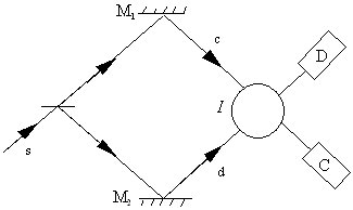
Figure 1: Simple interferometer
Although the predictions of experimental outcomes expressed in terms of probabilities are identical, Griffiths argues that, nevertheless, the two approaches actually give very different accounts of how a particle is supposed to pass through such an interferometer. After a detailed analysis of experiments based on figure 1 , he concludes that the CH approach gives a behaviour that is `physically acceptable', whereas the Bohm trajectories behave in a way that appears counter-intuitive and therefore `unacceptable'. This behaviour has even been called `surrealistic' by some authors 1 . Griffiths concludes that a particle is unlikely to actually behave in such a way so that one can conclude that the CH interpretation gives a `more acceptable' account of quantum phenomena.
Notice that these claims are being made in spite of the fact no new mathematical structure whatsoever is added to the quantum formalism in either CH or BI, and in consequence all the experimental predictions of both CH and BI are identical to those obtained from standard quantum mechanics. Clearly there is a problem here and the purpose of our paper is to explore how this difference arises. We will show that CH is not without its difficulties.
We should remark here in passing that these difficulties have already been brought out be Bassi and Ghirardi [8] [9] [10] and an answer has been given by Griffiths [11] . At this stage we will not take sides in this general debate. Instead will examine carefully how the analysis of the particle behaviour in CH when applied to the interferometer shown in figure 1 leads to difficulties similar to those highlighted by Bassi and Ghirardi [8] .
Let us first deal with the Bohm trajectory, which arises in the following way. If the particle satisfies the Schrödinger equation then the trajectories are identified with the one-parameter solutions of the real part of the Schrödinger equation obtained under polar decomposition of the wave function [4] . Clearly these one-parameter curves are mathematically well defined and unambiguous.
CH does not use the notion of a trajectory. It uses instead the concept of a history, which, again, is mathematically well defined to be a series of projection operators linked by Schrödinger evolution and satisfying a certainty consistency condition [1] . Although in general a history is not a trajectory, in the particular example considered by Griffiths, certain histories can be considered to provide approximate trajectories. For example, when particles are described by narrow wave packets, the history can be regarded as defining a kind of broad `trajectory' or `channel'. It is assumed that in the experiment shown in figure 1 , this channel is narrow enough to allow comparison with the Bohm trajectories.
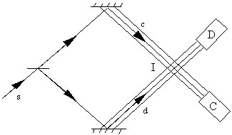
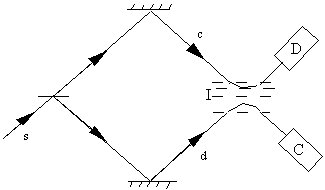
To bring out the apparent difference in the predictions of the two approaches, consider the interferometer shown in figure 1 . According to CH if we choose the correct framework, we can say that if C fires, the particle must have travelled along the path c to the detector and any other path is regarded as ``dynamically impossible" because it violates the consistency conditions. The type of trajectories that would be acceptable from this point of view are sketched in figure 2 . In contrast a pair of typical Bohm trajectories 2 are shown in figure 3 . Such trajectories are clearly not what we would expect from our experience in the classical world. Furthermore there appears, at least at first sight, to be no visible structure present that would `cause' the trajectories to be `reflected' in the region I, although in this region interference between the two beams is taking place.
In the Bohm approach, an additional potential, the quantum potential, appears in the region of interference and it is this potential that has a structure which `reflects' the trajectories as shown in figure 3 . (See Hiley et al. [7] for more details).
In this short note we will show that the conclusions reached by Griffiths [5] cannot be sustained and that it is not possible to conclude that the Bohm `trajectories' must be `unreliable' or `wrong'. We will show that CH cannot be used in this way and the conclusions drawn by Griffiths are not sound.
The transformation for t0® t
1 is
|
(1) |
The transformation for t1® t
2 is, according to Griffiths [13]
,[5]
|
(2) |
These lead to the histories
|
(3) |
These are not the only possible consistent histories but only these two
histories are used by Griffiths to make judgements about the Bohm trajectories.
The two other possible histories
|
(4) |
The significance of the histories described by equation (3) is that they
give rise to new conditional probabilities that cannot be obtained
from the Born probability rule [12]
. These conditional probabilities are
|
(5) |
Starting from a given initial state, y 0, these probabilities are interpreted as asserting that when the detector C is triggered at t2, one can be certain that, at the time t 1, the particle was in the channel c and not in the channel d. In other words when C fires we know that the triggering particle must have travelled down path c with certainty.
This is the key new result from which the difference between the predictions of CH and the Bohm approach arises. Furthermore it must be stressed that this result cannot be obtained from the Born probability rule and is claimed by Griffiths [12] to be a new result that does not appear in standard quantum theory 3 .
Looking again at figure 1 , we notice that there is a region I where the wave packets travelling down c and d overlap. Here interference can and does take place. In fact fringes will appear along any vertical plane in this region as can be easily demonstrated. Indeed this interference is exactly the same as that produced in a two-slit experiment. The only change is that the two slits have been replaced by two mirrors. Once this is realised alarm-bells should ring because the probabilities in (5) imply that we know with certainty through which slit the particle passed. Indeed equation (5) shows that the particles passing through the lower slit will arrive in the upper region of the fringe pattern, while those passing through the upper slit will arrive in the lower half 4 .
Recall that Griffiths claims CH provides a clear and consistent account of standard quantum mechanics, but the standard theory denies the possibility of knowing which path the particle took when interference is present. Thus the interpretation of equation (5) leads to a result that is not part of the standard quantum theory and in fact contradicts it. Nevertheless CH uses the authority of the standard approach to strengthen its case against the Bohm approach. Surely this cannot be correct.
Indeed Griffiths has already discussed the two-slit experiment in an earlier paper [14] . Here he argues that CH does not allow us to infer through which slit the particle passes. He writes; -
Given this choice at t3 [whether C or D fires], it is inconsistent to specify a decomposition at time t2 [our t 1] which specifies which slit the particle has passed through, i.e., by including the projector corresponding to the particle being in the region of space just behind the A slit [our c], and in another region just behind the B slit [our d]. That is (15) [the consistency condition] will not be satisfied if projectors of this type at time t2 [our t1 ] are used along with those mentioned earlier for time t3.The only essential difference between the two-slit experiment and the interferometer described by equation (3) above is in the position of the detectors. But according to CH measurement merely reveals what is already there, so that the position of the detector in the region I or beyond should not affect anything. Thus there appears to be a contradiction here.
To emphasise this difficulty we will spell out the contradiction again. The interferometer in figure 1 requires the amplitude of the incident beam to be split into two before the beams are brought back together again to overlap in the region I. This is exactly the same process occurring in the two-slit experiment. Yet in the two-slit experiment we are not allowed to infer through which slit the particle passed while retaining interference, whereas according to Griffiths we are allowed to talk about which mirror the particle is reflected off, presumably without also destroying the interference in the region I. We will return to this specific point again later.
One way of avoiding this contradiction is to assume the following: -
1. If we place our detectors in the arms c and d before the interference region I is reached then we have the consistent histories described in equation (3). Particles travelling down c will fire C, while those travelling down d will fire D. In this case we have an exact agreement with the Bohm trajectories.
2. If we place our detectors in the region of interference I then, according to Griffiths [14] , the histories described by equation (3) are no longer consistent. In this case CH can say nothing about trajectories.
3. If we place our detectors in the positions shown in figure 1 , then, according to Griffiths [14] , the consistent histories are described by equation (3) again. Here the conditional probabilities imply that all the particles travelling down c will always fire C. Bohm trajectories contradict this result and show that some of these particles will cause D to fire . These trajectories are shown in figure 3 .
It could be argued that this patchwork would violate the one-framework rule. Namely that one must either use the consistent histories described by equation (3) or use a set of consistent histories that do not allow us to infer off which mirror the particle was reflected. This latter would allow us to account for the interference effects that must appear in the region I.
A typical set of consistent histories that do not allow us to infer through which slit the particle passed can be constructed in the following way.
Introduce a new set of projection operators |
(c + d)ñá(c + d)
| at t3 where t1 < t3 < t
2. Then we have the following possible histories
|
(6) |
To bring out this problem let us first forget about theory and consider what actually happens experimentally as we move the detector C along a straight line towards the mirror M1. The detection rate will be constant as we move it towards the region I. Once it enters this region, we will find that its counting rate varies and will go through several zeros corresponding to the nodes in the interference pattern. Here we will assume that the detector is small enough to register these nodes.
Let us examine what happens to the conditional probabilities as the detector crosses the interference region. Initially according to (5), the first history gives the conditional probability Pr(c1 |y 0ÙC3 *) = 1. However, at the nodes this conditional probability cannot even be defined as Pr(C3*) = 0. Let us start again with the closely related conditional probability, derived from the same history Pr(C3 *|y0 Ù c1) = 1. Now this probability clearly cannot be continued across the interference region because Pr(C3* ) = 0 at the nodes, while Pr(y0 Ùc1) = 0.5 regardless of where the detector is placed. In fact, there is no consistent history that includes both c 1 and C3*, when the detector is in the interference region. We are thus forced to consider different consistent histories in different regions as we discussed above.
If we follow this prescription then when the detector C is placed on the mirror side of path c, before the beams cross at I, we can talk about trajectories and as stated above these trajectories agree with the corresponding Bohm trajectories. When C is moved right through and beyond the region I, we can again talk about trajectories. However in the intermediate region CH does not allow us to talk about trajectories. This means that we have no continuity across the region of interference and this lack of continuity means that it is not possible to conclude that any `trajectory' defined by y0Ä c1 ÄC* before C reaches the interference region is the same `trajectory' defined by the same expression after C has passed through the interference region. In other words we cannot conclude that any particle travelling down c will continue to travel in the same direction through the region of interference and emerge still travelling in the same direction to trigger detector C.
What this means is that CH cannot be used to draw any conclusions on the validity or otherwise of the Bohm trajectories. These latter trajectories are continuous throughout all regions. They are straight lines from the mirror until they reach the region I. They continue into the region of interference, but no longer travel in straight lines parallel to the initial their paths. They show `kinks' that are characteristic of interference-type bunching that is needed to account for the interference [15] . This bunching has the effect of changing the direction of the paths in such a way that some of them eventually end up travelling in straight lines towards detector D and not C as Griffiths would like them to do.
Indeed it is clear that the existence of the interference pattern means that any theory giving relevance to particle trajectories must give trajectories that do not move in straight lines directly through the region I. The particles must avoid the nodes in the interference pattern. CH offers us no reason why the trajectories on the mirror side of I should continue in the same general direction towards C on the other side of I. In order to match up trajectories we have to make some assumption of how the particles cross the region of interference. One cannot simply use classical intuition to help us through this region because classical intuition will not give interference fringes. Therefore we cannot conclude that the particles following the trajectories before they enter the region I are the same particles that follow the trajectories after they have emerged from that region. This requires a knowledge of how the particles cross the region I, a knowledge that is not supplied by CH.
Where the consistent histories (3) could provide a complete description is when the coherence between the two paths is destroyed. This could happen if a measurement involving some irreversible process was made in one of the beams. This would ensure that there was no interference occurring in the region I. In this case the trajectories would go straight through. This would mean that the conditional probabilities given in equation (5) would always be satisfied.
But in such a situation the Bohm trajectories would also go straight through. The particles coming from Mirror M1 would trigger the detector C no matter where it was placed. The reason for this behaviour in this case is because the wave function is no longer y c + yd, but we have two incoherent beams, one described by y c and the other by yd. This gives rise to a different quantum potential which does not cause the particles to be `reflected' in the region I. So here there is no disagreements with CH.
When the coherence between the two beams is preserved then CH must use the consistent histories described by equation (6). These histories do not allow any inferences about trajectories to be drawn. Although the consistent histories described by equation (3) enable us to make inferences about particle trajectories because, as we have shown they lead to disagreement with experiment. Unlike the situation in CH the Bohm approach can define the notion of a trajectory which is calculated from the real part of the Schrödinger equation under polar decomposition. These trajectories are well defined and continuous throughout the experiment including the region of interference. Since CH cannot make any meaningful statements about trajectories in this case it cannot be used to draw any significant conclusions concerning the validity or otherwise of the Bohm trajectories. Thus the claim by Griffiths [5] , namely, that the CH gives a more reasonable account of the behaviour of particle trajectories interference experiment shown in Figure 1 than that provided by the Bohm approach cannot be sustained.
2 Detailed examples of these trajectories will be found in Hiley, Callaghan and Maroney [7] .
3 It should be noted that the converse of (5) must also hold. Namely, if C does not fire then we can conclude that at t1 the particle was not in pathway c. In other words Pr(c1|y0 ÙC2) = 0
4 Notice that in criticising the Bohm approach, it is this consistent history interpreted as a `particle trajectory' that is contrasted with the Bohm trajectory. The Bohm approach reaches the opposite conclusion, namely, the particle that goes through the top slit stays in the top part of the interference pattern [15]