
|
Worksheet on using SPSS to analyse and compare cross-sectional developmental trajectories
The following worksheet steps through the use of SPSS to characterise cross-sectional developmental trajectories. In particular, we focus on comparing typically developing trajectories with those derived from a group of individuals with a developmental disorder. This worksheet accompanies the published paper:
Thomas, M. S. C., Annaz, D., Ansari, D., Serif, G., Jarrold, C., & Karmiloff-Smith, A. (2009). Using developmental trajectories to understand developmental disorders. Journal of Speech, Language, and Hearing Research, 52, 336-358. Click here for PDF version (837K).
To reference this worksheet, please cite the paper that it accompanies.
Conceptually, the following methods are very similar to standard Analyses of Variance (ANOVA). However, instead of testing the difference between group means, we are evaluating the difference between the straight lines used to depict the developmental trajectory in each group. While a group has a single number representing its average performance, it has two numbers representing its developmental trajectory - the intercept of the line (the level at which performance starts) and its gradient (the rate at which it increases or decreases with age). In the following sections, we introduce methods analogous to between-groups, repeated measures, and mixed-design ANOVAs but adapted for comparing developmental trajectories.
In the first section, we begin by characterising a single developmental trajectory, including generating and plotting confidence intervals around the trajectory, checking for outliers, assessing the linearity of the trajectory, and comparing goodness-of-fit of different linear and non-linear functions. Readers familiar with linear regression methods may wish to skip this section.
Focusing on the use of linear methods, we then introduce a between-groups comparison of trajectories that allows one to evaluate whether developmental trajectories generated from different groups differ significantly in terms of their gradients or intercepts. This employs a modified version of the traditional Analysis of Covariance (ANCOVA). We contrast comparisons between the groups for trajectories plotted according to chronological age with those plotted according to mental age measures.
In cases where the typically developing group produces a reliable trajectory but the disorder group does not, we offer a new method to distinguish between two different types of null trajectory in the disorder group: a zero trajectory, where there is no improvement with age in the disorder group; and no-systematic-relationship, where the task performance is essentially random with respect to the participant’s age. This is called the rotation method
In the third section, we show how SPSS can be used to compare two trajectories generated by a single group based on performance in two tasks in a repeated-measures design. With these trajectories, we also show how confidence intervals can be used to demonstrate the age at which the trajectories for the two tasks reliably converge or diverge.
In the fourth section, we demonstrate the use of SPSS to analyse mixed designs, e.g., with one between-groups factor and one repeated measure. For example, where the typically developing group is characterised by a divergence in development on two tasks, one might want to assess whether a disorder group demonstrates the same pattern of divergence.
Where appropriate, analyses are illustrated with worked examples using sample data. Charts are mostly generated within Excel and statistical results in SPSS 12.0 for Windows.
Some informal rules of thumb we have employed while using trajectory analyses can be found here. A recent paper by Annaz et al. (2009) demonstrating use of the methods can be found here.
1. Characterising a single developmental trajectory
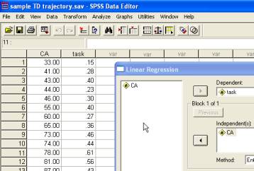
The sample data in sample TD trajectory.sav contain a single cross-sectional developmental trajectory for a sample of 25 typically developing children, aged from 2 years and 9 months (2;9) to 12 years and 5 months (12;5). The data depict the age in months of the children and the accuracy of their performance on a given experimental task across the age range.
The linear developmental trajectory, predicting task performance based on the chronological age of the children, is therefore
![]()
Here is an Excel chart of these data (employing the XY (Scatter) chart function; after the chart was created, the Add Trendline function under the Chart menu was used to add a best-fit linear trend; the Options tab in this dialogue permits display of the R2 value and the regression equation on the chart).
Illustrative Excel dialogues:
Several further pieces of information are important to explore a single trajectory. First, we wish to find out whether any of the data points exerts undue influence on the trajectory (i.e., constitutes an outlier). For this, we use Cook’s distance (Cook’s D). Second, we wish to assess the reliability of the parameters (the intercept and gradient). Third, we may wish to generate confidence intervals for the trajectory itself (i.e., the region within which the best-fit line falls with 95% confidence). To generate the additional bits of information, in the Linear Regression dialogue, click on the Statistics button and make sure both Estimates and Confidence intervals are selected. Click on the Save button and select Cook’s under Distances and Mean under Prediction Intervals (95% confidence is offered as the default value; this may be changed as desired). Then run the regression again.
The Save function in the dialogue has added three additional columns of data to the SPSS Data Editor. The first is Cook’s distance (COO_1). Cook’s D combines diagnostic information about Distance (useful for identifying potential outliers in the dependent variable, here Task) and Leverage (useful for identifying potential outliers in the independent variable, here CA) to identify unusually influential observations on the regression line (see Howell, 2007, p.516-520 for discussion). Cook’s D assesses how much the residuals of all cases would change if a particular case were to be excluded from the calculation of the regression coefficients (i.e. the total distance of all the points to the best-fit line). This is repeated for each case in turn; each data point can then be assigned a value measuring influence. There is no general rule for what value of Cook’s D definitively indicates that a given point is an outlier. However, as a rule of thumb, a Cook’s D of over 1.00 suggests that a data point exerts undue influence on the regression. In this case, the analysis should be re-run without the data point in question.
Note, however, that unless there are a priori grounds to exclude this participant’s data from the analysis (e.g., if an experimenter had noted at the time that a particular child may not have been paying attention during testing or there was an equipment malfunction), then the results must be reported for the analyses both with and without the identified data point(s). Treatment of variability in disorders is an important issue: behaviourally defined developmental disorders frequently exhibit marked variability, while variability is also found in disorders where an independent genetic diagnosis is available (see Thomas, 2003, for discussion and related analytical techniques). For the sample trajectory, no value of Cook’s D exceeds 0.2 and so no value is identified as a potential outlier.
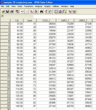
The two additional variables (LMCI_1, UMCI_1) created by the Save function are the lower mean confidence interval and the upper mean confidence interval for the dependent variable Task for each value of the predictor (i.e., for each age). The ‘mean’ confidence interval represents the region within which there is 95% chance that the actual mean (trendline) sits. Note that SPSS also gives you the option to save the ‘individual’ confidence intervals. These demarcate the region within which there is 95% probability that the individual data points will sit (these confidence intervals are typically wider).
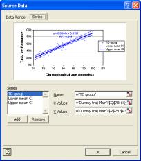
Confidence intervals can be added to the Excel chart by adding (CA, LMCI_1) and (CA, UMCI_1) as two additional X-Y scatter series. Click on your original chart to select it; under the Chart menu, select Chart-Source, select the Data-Series tab; click on the Add button and select the column of CA values and the column of LMCI_1 values as the X values and Y values respectively; repeat for CA and UMCI_1. To present these as thin lines as depicted below, select the data series (click on any point), right-click to Format data series, select None under Marker, and select Custom under Line, then select desired line format (thin, dotted, etc.). (Note that due to a bug in the charting function in Excel, we have sometimes found that the data series need to be ordered with the ages low-to-high on the spreadsheet for these to come out nicely. No idea why. This can be done by selecting the full chart data range, using the Data-Sort function, and sorting in ascending mode by the column that contains age).
Excel dialogue:
Lastly, in SPSS, selecting ‘confidence intervals’ under Statistics in the Linear Regression dialogue provides information on the upper and lower bounds of the intercept and gradient of the developmental trajectory. The results are shown in the below table. For our sample trajectory, since the upper and lower bounds of the confidence interval on the intercept span zero (-.076 to .102), this indicates that the intercept is not significantly different from zero (reflected in the non-significant t-test result on this coefficient). That is, it’s not clear whether the trajectory crosses the y-axis (where x=0) at a value where y is greater than 0 or less than 0. By contrast, the gradient is reliably greater than zero, indicating meaningful improvement with age.
Re-scaling the Age variable
In the following Sections, we sometimes re-scale the Age variable. For a single trajectory, we rescale age to the months from youngest age measured (mya). When comparing a typically developing trajectory and disorder trajectory, we rescale age to months from youngest disorder age measured (myda). This rescaling does not change the analysis but aids in interpretation.
In generating the equation for a linear regression, the intercept parameter tells us the value of the line when it crosses the y-axis, i.e., when age=0. In almost all cases, we will not have actually collected data at this age! More often, our data collection will span a band from some minimum age (or mental age) up to some maximum. Our description of the data has highest validity within this range and one must be extremely cautious extrapolating performance outside of the range.
In trajectory analyses, we often want to know what the level of performance is when we start measuring. When we talk about a presence or absence of delay at onset, we are talking about disparities in this initial level of measurement. It therefore makes much more sense to generate a linear regression whose intercept is calculated at the earliest age measured rather than age=0. To achieve this, we simply re-scale the age variable to count in months from the earliest age measured. For the current data, the earliest age measured is 33 months. Each CA is therefore recalculated to be (CA-33). When the linear regression is recalculated using the rescaled CA_mya as predictor, the equation is as follows:
![]()
While the gradient remains the same (we have only re-scaled the Age variable), the intercept now corresponds to the value at which the trajectory begins (21%; see Excel plot above). For comparisons between a typically developing trajectory and a disorder trajectory, usually we want to know whether there is a disparity between the groups at the earliest age (or mental age) measured for the disorder group. Hence this is the age used to do the rescaling. For more details, see here.

Linearity and model comparison
The sample data represent a trajectory that is reasonably linear. What if we are not confident that a simple line gives a best fit to the data? We can, of course, check that the residuals (the difference between the actual performance of each individual and the performance that is predicted by the trajectory given each individual’s age) are normally distributed and do not vary systematically across the age range. These indicators (along with the R2) would warn if a linear function does not capture the cross-sectional trajectory very well. SPSS, however, also allows us to assess whether another non-linear function fits the data better.
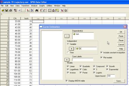
SPSS permits multiple functions to be simultaneously fitted to the same set of data points using the Analyze-Regression-Curve Estimation Function. Parameter information and proportion of variance explained can be derived for several functions at once, linking performance (Y) to age (t) using parameters b0, b1, b2 . . . in the following ways:
(Taken from SPSS 12.0 for Windows help function under ‘Curve
Estimation’)
· Linear. Model
whose equation is Y = b0 + (b1 * t). The series values are modeled as a linear
function of time
· Logarithmic. Model
whose equation is Y = b0 + (b1 * ln(t))
· Inverse. Model
whose equation is Y = b0 + (b1 / t)
· Quadratic. Model
whose equation is Y = b0 + (b1 * t) + (b2 * t**2). The quadratic model can be
used to model a series which "takes off" or a series which dampens
· Cubic. Model
defined by the equation Y = b0 + (b1 * t) + (b2 * t**2) + (b3 * t**3)
· Power. Model
whose equation is Y = b0 * (t**b1) or ln(Y) = ln(b0) + (b1 * ln(t))
· Compound. Model
whose equation is Y = b0 * (b1**t) or ln(Y) = ln(b0) + (ln(b1) * t)
· S-curve. Model
whose equation is Y = e**(b0 + (b1/t)) or ln(Y) = b0 + (b1/t)
· Logistic. Model
whose equation is Y = 1 / (1/u + (b0 * (b1**t))) or ln(1/y-1/u)= ln (b0) +
(ln(b1)*t) where u is the upper boundary value. After selecting Logistic,
specify the upper boundary value to use in the regression equation. The value must be a positive number, greater than the largest
dependent variable value [for our sample data, the largest value of Task is in
principle 100, so one might choose 101 for the boundary value]
· Growth. Model
whose equation is Y = e**(b0 + (b1 * t)) or ln(Y) = b0 + (b1 * t)
· Exponential. Model
whose equation is Y = b0 * (e**(b1 * t)) or ln(Y) = ln(b0) + (b1 * t)
A plot of these fits can also be obtained by clicking on the Plot models box:
For our sample trajectory, most of the functions give a reliable fit to the data. Here are their R2 (taken from the ANOVA table for each function in the SPSS output; see below):
|
Function |
R2 |
Number of
parameters estimated (b0, b1, etc.) |
|
Linear |
.87972 |
2 |
|
Logarithmic |
.84760 |
2 |
|
Inverse |
.75463 |
2 |
|
Quadratic |
.87975 |
3 |
|
Cubic |
.87979 |
4 |
|
Compound |
.81382 |
2 |
|
Power |
.85834 |
2 |
|
S |
.84181 |
2 |
|
Growth |
.81382 |
2 |
|
Exponential |
.81382 |
2 |
|
Logistic |
.81435 |
2 |
Cubic gives the highest R2, while Compound, Growth, and Exponential give the lowest.
How do we decide which is the best function to fit the data? Here, the heuristic of parsimony comes in. We want to explain the most amount of variance using the least number of parameters. For example, although the Quadratic function fits the data better than the Linear (i.e., has a larger R2), it does so with one more parameter; the Cubic fits marginally better than the Quadratic but uses one more parameter again.
There are two statistical tests that can be used to determine which model/function to choose in these cases. One method, called the ‘extra sum-of-squares’ test, is only applicable for nested models. A nested model is one where one model is a subset of the other, that is, the first model is a version of the second model but with one or more of the parameters set to zero. Thus the Linear model is a version of the Quadratic model with the x2 coefficient set to zero, and a version of the Cubic model with the x2 and x3 coefficients set to zero. Nested models will have different degrees of freedom. The extra sum-of-squares approach derives an F-ratio from the relative increase in the sum-of-squares and the relative increase in the degrees of freedom reflecting the number of parameters used (this information is available in the ANOVA table for each regression fit). These two values are played off against each other, where an increase in model fit is good and an increase in parameters is bad. For regression fits 1 and 2 (where 1 is the simpler model with fewer parameters), the equation is
![]()
where SS stands for sum-of-squares and DF for degrees of freedom. This F-ratio has DF1-DF2 degrees of freedom for the numerator and DF2 degrees of freedom for the denominator (see Motulsky & Christopoulos, 2004, for more details).
For example, let us compare the Linear and Cubic fits to the sample data. The SPSS printouts provide the sum-of-squares and degrees-of-freedom information (relevant information highlighted in blue):
Dependent variable.. task Method.. LINEAR
Listwise Deletion of Missing Data
Multiple R .93793
R Square .87972
Adjusted R Square .87449
Standard Error .07629
Analysis of Variance:
DF Sum of
Squares Mean Square
Regression 1 .97897124 .97897124
Residuals 23
.13385276
.00581969
F =
168.21722 Signif F = .0000
-------------------- Variables in the
Equation --------------------
Variable B
SE B Beta T
Sig T
CA .006060
.000467 .937933 12.970
.0000
(Constant) .013136
.043018 .305 .7628
Dependent variable.. task Method.. CUBIC
Listwise Deletion of Missing Data
Multiple R .93797
R Square .87979
Adjusted R Square .86261
Standard Error .07981
Analysis of Variance:
DF Sum of
Squares Mean Square
Regression 3
.97904851 .32634950
Residuals 21
.13377549
.00637026
F =
51.23016 Signif F = .0000
-------------------- Variables in the
Equation --------------------
Variable B
SE B Beta T
Sig T
CA .007201
.011874 1.114523 .606
.5507
CA**2
-1.254574265500E-05
.000141 -.351645 -.089
.9298
CA**3
4.212775775628E-08
5.1479E-07 .179103 .082
.9356
(Constant) -.017479
.303698 -.058 .9546
_
For this model comparison, an F-test produces the following outcome: F(2,21)=.006, p=.994. This indicates that the greater number of parameters in the Cubic model is much more expensive than the slightly greater fit to the data that the function provides. Therefore the simpler Linear model is the better model.
For non-nested models, the ‘extra sum-of-squares’ method is not applicable. This becomes evident if one tries to compare models that have the same number of parameters. The formula requires the denominator to calculate the difference in degrees of freedom but the difference (DF1-DF2) is now zero. Division by zero generally causes things to go badly wrong.
In the case of non-nested models, one can replace a hypothesis testing approach to comparing the models with an approach one drawn from information theory. This technique employs Akaike’s Information Criterion (see Motulsky & Christopoulos, 2004, p.143, for further details). In the hypothesis testing approach, the result of the test indicates the likelihood of the more complicated model happening to better fit the data just by chance. In the information theory approach, the test instead computes the relative likelihood of each model being correct.
The Akaike’s Information Criterion (AIC) for each model is
![]()
where N is the number of data points, K is the number of parameters fit by the regression plus one, and SS is the sum of the squares value taken from the regression equation. Let us compare the AIC scores for the Linear and Logistic models for the sample data, both of which fit two parameters (‘CA’ and ‘constant’ below).
Dependent variable.. task Method.. LGSTIC
Listwise Deletion of Missing Data
Multiple R .90241
R Square .81435
Adjusted R Square .80628
Standard Error .20389
Analysis of Variance:
DF Sum of
Squares Mean Square
Regression 1 4.1941911 4.1941911
Residuals 23 .9561769 .0415729
F =
100.88760 Signif F = .0000
-------------------- Variables in the
Equation --------------------
Variable B
SE B Beta
T Sig T
CA
.987535
.001233 .405590 800.739
.0000
(Constant) 6.000506 .689910
8.698 .0000
Applying the equation,
- AIC for Linear fit = -124.7
- AIC for Logistic fit = -75.6
The model with the smallest AIC value is most likely to be correct – in this case, the Linear model.
Excel formulae for computing the extra sum-of-squares test and Akaike’s Information Criterion can be found here (including use of corrected AIC values and a method to compute the relative probability that you are correct if you choose one or other model).
What do you do if a non-linear function provides a better fit to the data? In the following, we focus on linear methods to compare trajectories. The primary motivation for this is that linear methods render interaction terms more interpretable and thus allow us to distinguish different types of descriptive delays. It is a practical rather than a theoretical decision – there is no requirement that development should proceed at a constant rate and in many cases it does not (e.g., the rate of vocabulary acquisition is children is famously non-linear). However, the methods that we present for use with linear functions are in principle extendible to non-linear regression methods, where for example, differences in the intercept parameter can index delays in onset and differences in other parameters can index differences in rates of non-linear growth (see Motulsky & Christopoulos, 2004, for a review of non-linear regression methods with biological data).
Linear methods may be used in cases where the relationship between age and performance is non-linear by transforming either or both of these dimensions to improve the linearity of the relationship between them (so long as the transformation is applied to both typical and disorder group). Thus an S-shaped or sigmoid function can be linearised via a probit transform (see Jarrold, Baddeley & Phillips, 2007). Reaction time changes are frequently non-linear across age. Plotting the log of reaction time against the log of age can linearise this function.
Alternatively, subsections of the full non-linear trajectory may be explored where development appears to be more linear. For example, in cases where there are early floor or late ceiling effects, the portion of the trajectory between floor and ceiling may be more linear. Thus, for an S-shaped curve, only the central part of the trajectory might be considered with linear methods. The more restricted analysis would allow one to identify differences in the average age that experimental groups reach ceiling performance on the task. Analyses run over subsets of the experimental group will, of course, compromise statistical power.
We now turn to consider methods to compare the developmental trajectory generated by a disorder group to the typically developing profile.
2. Between-group comparisons of two developmental
trajectories
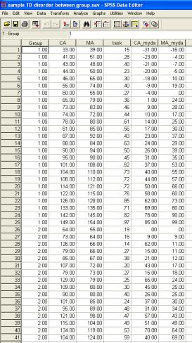
The SPSS data file sample TD disorder between group.sav contains data for two groups, the typically developing (TD) group of 25 children with ages spanning from 2;9 to 12;5, and a group of 16 children with a developmental disorder with chronological ages ranging from 5;4 to 11;2. Note that all children have also been given a standardised test to produce a mental age (i.e., a test age equivalent score).
For the TD group, their mental ages range from 3;3 to 12;10, with the average MA 4.7 months in advance of CA (that is, the performance of this typical sample is in advance of the sample of TD children on whom the standardised test was normed. Information about sampling would be required to decide whether the TD or norming sample is in some sense any more or less ‘normal’).
For the disorder group, MAs range from 4;7 to 10;4, with the average MA 18.1 months behind CA. In the SPSS file, group is encoded with the Group variable (coded 1 for TD, 2 for disorder in our example). CA and MA are coded in months and task performance is coded in proportion correct on the experimental task (ignore CA_myda and MA_myda for the time being).
Note that, by design, the TD group’s age range spans from the youngest mental age of the disorder group on any of the standardised tests used to assess this group, to the oldest CA of the disorder group. This is because it is only sensible to compare developmental trajectories for overlapping chronological or mental age ranges. Comparing non-overlapping trajectories necessitates extrapolating a prediction of task performance for one or other group outside of the age or ability range over which performance has been measured.
Charting in Excel, these trajectories are as follows:
Are the individuals with the disorder performing on the task as you would expect given their chronological age? One way to answer this question is on a case-by-case basis. This can be done using the confidence intervals around the TD trajectory derived in the previous section. For each child with the disorder, we can see whether, when their performance is plotted on the chart according to their chronological age, the data point falls within the 95% confidence intervals around the TD trajectory.
However, our intention here is to characterise a developmental trajectory for the disorder group as a whole, given that we have reasonable participant numbers (N=16) across an age range and our aim is to characterise the disorder. We therefore need to generate a trajectory for the disorder group and compare it to the TD trajectory. Are the two trajectories significantly different, and if so, in what way?
SPSS does not include a direct method to compare linear regressions. Instead, we will adapt the Analysis of Covariance function within the General Linear Model (ANCOVA). This method is equivalent to including dummy variables in a linear regression model to assess the significance of dichotomous / categorical variables and their interaction with continuous variables (see Suits, 1957). An alternative (though conceptually identical) approach is to use multiple regression models (e.g., Brock & Jarrold, 2004; see Wright, 1997, p.185-186).
Assuming we have already verified the approximate linearity of the disorder trajectory on its own, we begin by comparing the developmental trajectories for the two groups as they are predicted by chronological age.
We now come to a slight complication, albeit one of interpretation. One of our aims will be to compare the intercept values of the two trajectories (equivalent to a main effect of Group in the following analyses). The rationale to do this is to establish a possible delay in onset in the disorder group, where onset is defined as the level of performance observed at the earliest age measured on the task, and delayed onset is defined as any difference between the performance of the two groups when measurement starts. However, when we compare the intercepts of two trajectories, the comparison is carried out at the point where the lines cross the y-axis (i.e., at age=0 months). This makes little sense conceptually; it compares the trajectories outside of the age range over which we have measured behaviour.
In order to correct for this, we re-scale the x-axis, so that it measures age in months from the youngest age measured in the disorder group. This means that the difference between two trajectories will now be calculated at the point where measurement began (the green line on the plot below). For more details on re-scaling the age variable, and specifically, which age you should use as the 'zero' age, see here.
The SPSS data sheet therefore contains two additional variables. CA_myda and MA_myda, where myda stands months from youngest disorder age measured. For CA, the youngest disorder age measured is 64. CA_myda is therefore (CA-64). For MA, the youngest disorder age measured is 55. MA_myda is therefore (MA-55).
Note that changing the scale of the age variable in this way has no effect on the analyses, other than specifying the age at which the main effect of Group is calculated. And we carry out this rescaling only to aid the theoretical interpretation of group differences with regard to delays in onset.
To carry out the comparison of trajectories, select Analyze-General Linear Model-Univariate. Add Task to the Dependent Variable box, Group to the Fixed Factor(s) box, and CA to the Covariate(s) box. (The Save dialogue may be used to generate Cook’s D values for the two trajectories if this has not been done previously).
We must do one more thing before we run the analysis and that is to specify the appropriate effects within the model. The SPSS ANCOVA function has a default design in which it tests for a main effect of Group and a main effect of the covariate (Age), but not for an interaction between Group and the covariate (Group x Age). Why is this? The normal design of the between-groups ANCOVA attempts to test for a difference between the groups correcting for any difference the groups may have on the covariate. For instance, if Group 1 is older than Group 2, you might expect Group 1 to score better than Group 2 anyway. How can we tell if Group 1 is performing better than Group 2 independent of their difference in age? The way the ANCOVA answers this question is to compute a single regression function relating performance and age from both groups combined, then use this regression equation to adjust the performance scores of each group to compensate for their difference in mean ages. Any performance difference that remains after the adjustment is assumed to reflect an underlying group difference. The technique means that the normal ANCOVA relies on the assumption that the gradient of the two trajectories is the same, since the adjustment is done on the basis of a single overall regression between performance and age (see Howell, 2007, p.590). Violations of this assumption undermine use of the normal ANCOVA model.
In our case, however, we are explicitly testing the hypothesis that the gradient of the two regressions is different, that is, that the typically developing and disorder groups are developing at different rates. Therefore, we need to add the interaction term of (Group x Age) to the model. This turns out to be a relatively simple procedure.
We add the Group x Age interaction term to the model as follows. Click on the Model button in the Univariate dialogue. In the Model dialogue, select Custom. Set the Build Terms drop down to Main effects. Click on Group(F) and CA_myda(C) and use the right arrow button to move these across to the Model box. (Nb., the F and C stand for Fixed and Covariate, respectively). Then set the Build Terms drop down to Interaction. Select both Group(F) and CA_myda(C) by clicking on them in turn, and then click on the right arrow button to add this interaction term to the model. The dialogue box should now look like this:

Click on Continue, and then run the analysis by clicking on OK in the main Univariate dialogue.
Two results tables are now of interest. The Tests of Between-Subjects-Effects allows us to assess how much of the variance in the data we have explained. The overall R2 is .774 (calculated by dividing the sum-of-squares for the Error, .409, by the Corrected Total sum-of-squares, 1.809, and subtracting the result from 1). The model explains a significant proportion of this variance [F(3, 37)=42.23, p<.001, η2=.774]. The partial-eta-squared (η2) statistic here corresponds to the effect size for the analysis (see Howell, 2007, p.585, for discussion).
Inspection of the results for each factor indicate that there is an overall effect of Group [F(1, 37)=5.95, p=.020, η2=.139]. This tells us that the intercepts of the two groups are reliably different at the youngest age of measurement in the disorder group. The disorder group therefore exhibits a Delayed Onset in development.
With the groups combined, chronological age significantly predicts level of performance [F(1, 37)=32.88, p<.001, η2=.470]. However, there is also a significant Group X CA_myda interaction. The disorder group is developing more slowly on this task [F(1, 37)=7.40, p=.010, η2=.167]. They are also exhibiting a Slower Rate of development.
As with the traditional use of Analysis of Variance, one must be cautious in interpreting main effects where significant interactions are present. For example, in the extreme case illustrated below, there would be no main effect of Group (trajectories intercept at the y-axis), no main effect of Age (grand average trajectory has a gradient of zero), but a reliable interaction between the trajectories. Results therefore must always be interpreted with reference to the plotted data.
The Parameter Estimates table allows us to reconstruct the regression equations for the two trajectories (and include confidence intervals on these estimates). These parameters allow us to quantify the difference between the trajectories.
In interpreting this table, note that SPSS selects one group to have the derived values of the intercept and gradient (i.e., rate of change against the predictor: CA_myda), and then provides a modifier to these values if the group membership is different. Thus the intercept for the disorder group (Group 2) is .256 and the gradient is .002, while the intercept for the TD group (Group 1) is (.256+.145)=.401 and the gradient is (.002+.004)=.006.
The parameter values should correspond to the those generated by carrying out individual linear regressions for each trajectory in SPSS or by using Excel’s trendline fitting algorithm in the X-Y Scatter-plot Chart (so long as the CA_myda variable has been used as the predictor). Comparison of analyses employing CA as the predictor instead of the re-scaled CA_myda should confirm that the intercept is altered by the re-scaling but the gradient remains the same.
The two regression equations are as follows:
![]()
![]()
In terms of slower rate, we can straightforwardly say that the disorder group is developing at a third of the rate of the TD group (i.e., .002/.006=.333).
In terms of the delayed onset, we can report this difference in one of two ways. We can either
(a) report the performance difference at the youngest age measured, that is, the difference between the intercepts. This corresponds to a 15% disparity in accuracy at onset [.401-.256=.145];
or
(b) report the age difference at the lowest performance of the disorder group. This corresponds to a test age difference of 24 months [predicted performance at youngest age: .256; age for TD trajectory at which performance is .256: (+.256-.401)/.006 = -24.17 months].
Plotting performance against mental age
The analysis so far has indicated that the disorder group is not at a level we would expect given their chronological age. In some cases, this is unsurprising for a disorder, particularly if we are examining an area of apparent weakness (such as reading in developmental dyslexia). In other cases, the CA analysis may be central, such as when we believe we are examining an area of potential strength or normal development in the disorder (e.g., non-verbal reasoning in developmental dyslexia).
Given that performance is not at CA level in the disorder group, our next question becomes: is the performance of the disorder group at a level we would expect given their level of cognitive development, as measured by our selected standardised test? If we plotted the disorder trajectory according to mental age (MA) rather than CA, would the disorder trajectory now fall on top of the TD trajectory?
Note that this is a theory-dependent comparison, because it relies on us having made the right theoretically motivated choice about which standardised test is appropriate to evaluate the level of cognitive development in the domain that pertains to our experimental task (e.g., to generate MAs for a disorder group in an experimental task investigating sentence repetition, one might use a test of receptive grammar such as the TROG; one might, more tentatively, use the Matrices test of non-verbal reasoning; one might be less likely to use a block design or face recognition test – although one could of course try).
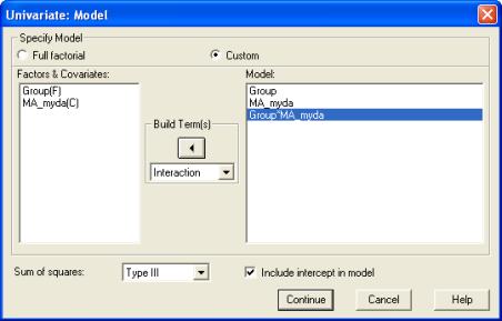
To carry out this second comparison, we run the statistical test again, but now substituting MA_myda as the covariate (where ‘MA_myda’ is the youngest mental age measured in the disorder group). Remember, this requires that we re-specify the Custom model to include the following factors: Group, MA_myda, and Group*MA_myda:
When task performance is plotted against the unscaled MA scores, the trajectories look like this:
Again, the vertical green line reflects the age at which the group comparison will be carried out when the MA data are rescaled.
The results of comparing disorder and TD trajectories based on MA_myda yield the following SPSS results tables:
As suggested by the data plot, the two trajectories are now parallel: there is no reliable interaction of Group x Age [F(1, 37)=.21, p=.885, η2=.001]. Mental age is a strong predictor of performance over all participants [F(1, 37)=127.29, p<.001, η2=.775]. However, a reliable group difference remains [F(1, 37)=12.05, p=.001, η2=.246].
In short, while the rate of development is normalised by plotting the disorder trajectory according to MA, the onset is not. Performance on the task is developing in line with the rate of general development in this domain but suffered a delay in onset compared to general development in the domain.
Note, even if this MA analysis had revealed no reliable differences between the groups in onset or rate, we could not say that the disorder group is developing normally on this task. This is because we have already established in the CA analysis that the disorder group is developing at a slower rate and with a delayed onset. The MA analysis would have merely demonstrated that these differences were in keeping with the developmental pattern exhibited in this domain as a whole by the disorder (to the extent that the standardised test we have chosen is a valid measure of the domain).
Comparing CA- and MA-based trajectories
Note that if we examine the disorder group trajectories in isolation, the R2 value increases from 0.104 for the CA plot [F(1, 14)=1.60, p=.227, η2=.103] to 0.76 for the MA plot [F(1, 14)=42.37, p<.001, η2=.752]. For disorders with learning disability, this is a frequently observed pattern. Where the standardised test is indeed relevant to the experimental task, or where the standardised test loads heavily on the general factor of intelligence (such as Ravens matrices), MA will usually be a better predictor of task performance than CA. This is especially the case in a cross-sectional design, where the severity of an individual’s disorder may not correspond closely to his or her age (especially if, for example, the oldest individuals happen, by chance sampling, to have the most severe cases of the disorder). In a longitudinal design, MA and CA may correlate more strongly and therefore their predictive power may be more equal. (See main paper for a theoretical discussion of the predictive power of CA vs. MA).
For the disorder group in our sample data, the correlation between CA and MA was only 0.58. Stepwise regression indicates that MA predicts reliably more of the variance in task performance than CA [R2 produced by entering both CA and MA into the linear model = .805, F(2, 13)=26.78, p<.001; R2 change produced by removing MA = .702, F(1, 13)=46.73, p<.001].
One disadvantage of entering CA and MA as predictors in the same regression is the possibility of multicollinearity artefacts (i.e., both predicting the same variance). Other methods for comparing CA and MA-based analyses include examining the confidence intervals on the parameters of the regression equations to see whether they overlap. They may be compared more directly by including age_type as an additional factor in a between-subjects comparison (ensuring all 2-way and 3-way interactions are specified in the Custom model), although this is a conservative comparison since the two trajectories are treated as between- rather than repeated measures. We won’t go into any further details on these analyses here.
A note on omnibus comparisons versus individual group comparisons
The following situation can sometimes occur. When the TD trajectory is characterised in isolation, age reliably predicts performance, albeit with a small effect size. When the disorder group is characterised in isolation, age does not reliably predict performance. However, when both TD and disorder groups are combined in a single omnibus comparison (with group added as a between-participants factor), not only does age not predict performance overall, but there is also no group*age interaction (as you might expect if age were a reliable predictor in only one group). The usual reason for this is that there is unequal variance in the two groups. For example, if there is much greater variability in the disorder group than the TD group, this greater background noise washes out any small effects observed only in the TD group (since the disorder group's variability is adding to the sum of variability to be explained).
Under these circumstances, we believe it correct to report the patterns observed in the groups in isolation (since these are planned comparisons - one is assessing the developmental profile of each group before comparing them). One should also note that effects are absent in the overall omnibus comparisons. It is important, however, to verify what it is about the structure of the data that is leading to the problem with t he omnibus comparison (e.g., unequal variance between the groups).
Interpreting null trajectories in the disorder group
On occasions, although age reliably predicts performance in the TD group, there may be no significant relationship in the disorder group. This can occur for two different reasons. Either performance is simply not changing with age (e.g., the disorder group have got as good as they are going to get on this type of task); or performance in the disorder group is essentially random with respect to age. It is possible to distinguish between these two possibilities statistically. Our technique uses the variability in the TD group as a benchmark to determine how much variability one would expect in the disorder group under each possibility. The rotation method for interpreting null trajectories in the disorder group and, more specifically, for distinguishing between the cases of zero trajectory and no systematic relationship, can be found here.
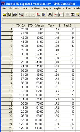
The SPSS data file sample TD repeated measures.sav contains performance data for the typically developing (TD) group of 25 children (ages 2;9 to 12;5) on two experimental tasks.
The respective trajectories are:
The analysis proceeds in two phases. First we use an analysis that omits the covariate to explore the within-subjects effects (i.e., the main effect of Task). This reduces the model to a repeated-measures ANOVA. Second, we add the covariate (age) and re-run the analysis as an ANCOVA; we use the results from this analysis to explore the effects of the covariate and the interaction of the covariate with the within-subjects factor (task*age). The reasons for the separate analyses are a little complicated and can be found here.
Phase 1. To compare the effects of the repeated measure of Task, select Analyze-General Linear Model-Repeated Measures. Define a Within-Subject Factor ‘task’ with two levels. Click on Define. In the Repeated Measures dialogue, add the two variables Task1 and Task2 as Within-Subjects Variables. Select Estimates of effect size and Parameter Estimates in the Options dialogue. Then run the analysis by clicking on OK in the Repeated Measures dialogue.
The results of this comparison show a clear main effect: children in the TD group are better at Task 2 than Task 1 [F(1, 24)=26.61, p<.001, η2=.526]
In the parameter estimates table, the intercepts reflect the means of the group’s performance on Task 1 (53.5%) and Task 2 (67.2%), along with the confidence intervals and effect sizes.

Reader query: Why have you used Within-Subjects Contrasts here, rather than Within-Subjects Effects?
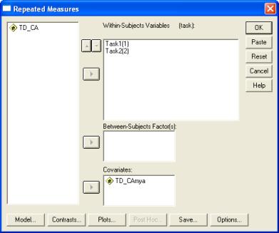
Phase 2: Once more, in order to assess the difference between the trajectories at their onset, we compute a new version of the covariate, which is the age in months from youngest age measured (TD_CAmya). The youngest age for this sample is 33 months. Each CA is rescaled to be (CA-33) months.
Now we add the covariate to the design. Select Analyze-General Linear Model-Repeated Measures. Click on Define and in the Repeated Measures dialogue, add the TD_CAmya as the covariate. Estimates of effect size and Parameter Estimates should still be selected in the Options dialogue. Cook’s distance information may also be generated using the Save dialogue, to check for outliers around each trajectory. Then run the analysis by clicking on OK in the Repeated Measures dialogue. (No custom model needs to be specified here. SPSS’s default model contains all the relevant terms).
The SPSS output tables are as follows:
Overall, performance significantly improves with age [F(1, 23)=197.52, p<.001, η2=.896]. There is a marginally significant interaction between age and task [F(1, 23)=3.88, p=.061, η2=.144], suggesting a difference in the rate of development on the two tasks.
Since 100% is the maximum score in both tasks, there is a possibility that this interaction stems from a ceiling effect for Task 2. The performance advantage of 20% for Task 2 over Task 1 at around 30 months could not be replicated at 150 months (the oldest age measured) since Task 1 is already at 90% and therefore Task 2 would have to exceed the ceiling score. (One could verify this interpretation by re-running the analysis for a subset of the sample, say for children below 120 months.)
Finally, the Parameter Estimates provide the coefficients for trajectories two separate task trajectories in the TD group.
In sum, trajectory analysis within the group suggests reliably higher performance at onset for Task 2 but a (marginally reliable) slower rate of development, perhaps the result of a ceiling effect on Task 2.
Using confidence intervals to assess when trajectories diverge/converge
In some circumstances, theory predicts that trajectories should converge or diverge. For instance, as children get better at recognising faces, they find it increasingly hard to detect differences in faces when they are presented upside-down. Therefore, normal development should produce an increasing trajectory of accuracy in upright face recognition and a decreasing trajectory of accuracy in inverted face recognition. This is the pattern that has been observed in trajectory analysis for children between 6 and 12 years of age (Annaz, 2006). In cases like this, it may be useful to derive the age at which two trajectories reliably diverge. This can be achieved by plotting the trajectories for the two tasks (or two groups for a between-participants comparison) along with their 95% confidence intervals. The confidence intervals can be generated using the linear regression function for each trajectory on its own (see section 1). The point at which the upper confidence interval of the lower trajectory and the lower confidence interval of the higher trajectory cease to overlap provides an estimate of the age (or mental age) at which the trajectories diverge. Of course, 95% confidence limits represent an arbitrary convention on the reliability of differences, so the divergence / convergence point should not be over-interpreted.
The following plot illustrates the method for the repeated measures TD sample data. It indicates that the trajectories for the two tasks reliably converge above the age of 114 months.
The SPSS data file sample TD disorder mixed design.sav contains performance data for the typically developing (TD) group of 25 children (ages 2;9 to 12;5) and the 16 children in the disorder group (ages 5;4 to 11;2) on two experimental tasks. We will therefore be constructing and comparing four developmental trajectories, two for each group.
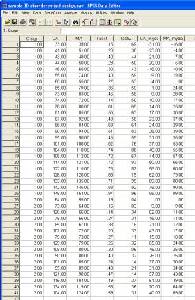
The four trajectories constructed according to chronological age are as follows (the green line again indicates the youngest disorder age measured):
We can assess the performance of the disorder group on an individual-by-individual basis using the confidence intervals around the two TD trajectories. Say that a given individual from the disorder group scores at 20% on Task 1 and 33% on Task 2, a disparity of 13%. We can evaluate whether this pattern (20, 33) is found anywhere across the TD trajectories, with each point inside the respective TD trajectory’s confidence intervals; or, indeed, whether the disparity size of 13% is found anywhere across the TD trajectories. These questions can be answered irrespective at the age at which any such patterns are exhibited in the TD group. This is a theory-neutral comparison of individuals with the disorder to the normal pattern of development. However, as before, our primary interest lies with group comparisons.
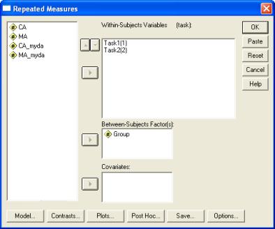
To compare these trajectories statistically, we need to construct a mixed-design model in SPSS, with Group as a between-participants factor and Task as a within-participants factor. As in Section 3, we can examine the main effect of the repeated measures Task effect in a separate ANOVA. Select Analyze-General Linear Model-Repeated Measures. Define a Within-Subject Factor ‘task’ with two levels. Click on Define.
The results are as follows:
There is no main effect of Task [F(1, 39)=.33, p=.569, η2=.008]. However, as we indicated earlier, this comparison collapses across groups and may be misleading. Indeed, there is a strong interaction with Group, reflecting the fact that in the TD group, performance on Task 2 is better than on Task 1 while in the disorder group performance on Task 1 is better than on Task 2. (Analysis of the disorder group in isolation reveals that this reverse task effect is indeed reliable [F(1, 15)=8.78, p=.010, η2=.369]). However, the Task*Group interaction we will report will come from the ANCOVA analysis, since the groups may differ on their age or mental age; addition of the covariate will adjust for these differences in evaluating the Task*Group interaction.
Now we add the covariate to the design. Select Analyze-General Linear Model-Repeated Measures. Click on Define and in the Repeated Measures dialogue, add the CA_myda (CA rescaled as months from youngest disorder age measured) as the covariate. Estimates of effect size and Parameter Estimates should still be selected in the Options dialogue. Cook’s distance information may also be generated using the Save dialogue, to check for outliers around each trajectory.
As with the between-subjects comparison, the default SPSS ANCOVA design unfortunately does not include all the requisite interaction terms. In this case, it omits the interaction between the covariate CA_myda and the between-subjects factor of Group. As in Section 2, we use the Model dialogue to add this term to the analysis. Specify a Custom model. Select Main effects in the Build Terms dropdown menu, then highlight each of the factors Task, Group, and CA_myda(C) in turn and use the right arrow to transfer them to the Within-Subjects Model box and Between-Subjects Model box, respectively. Then select Interactions (or All 2-way does the same thing here) from the Build Terms dropdown menu, highlight Group and CA_myda(C) by clicking on them, and then the right arrow to transfer the CA_myda*Group interaction term to the Between-Subjects Model box. Then click on Continue and run the analyses by clicking on OK in the Repeated Measures dialogue.
The results are as follows.
To interpret these results, we start with the key theoretical question: Does the disorder group show the same developmental relationship between the two tasks as that found in the TD group?
This corresponds to a 3-way interaction between task x Group x CA_myda. The answer is yes, for this interaction is non-significant [F(1, 37)=2.11, p=.155, η2=.054]. However, the two groups do show a different pattern of accuracy on each task, with the TD group performing more accurately on Task 2 than Task 1, while the disorder group performs more accurately on Task 1 than 2 [task x Group: F(1, 37)=17.70, p<.001, η2=.324]. Overall, the disorder group shows a delayed onset, demonstrated by a main effect of Group [F(1, 37)=51.18, p<.001, η2=.580]. Chronological age is a strong predictor of performance overall [CA_myda: F(1, 37)=60.15, p<.001, η2=.619] but development once again occurs more slowly in the disorder group than the TD group [Group x CA_myda: F(1, 37)=6.06, p=.019, η2=.141].
The Parameter Estimates table allows the equations for each of the four trajectories to be constructed. Parameters are listed separately for each task. Within the task, the default intercept and gradient (onset and rate) are listed for Group 2, with Group 1 values corresponding to modifiers to these default values. These parameter values should correspond to the regression equations on the Excel Scatter-plot chart trendlines if CA_myda is used as a predictor. Where CA is used as a predictor, the Excel charts should generate trendlines with the same gradients but different intercepts (since those intercepts are calculated at age=0 rather than the youngest age of the disorder group).
Plotting performance against mental age
Next we want to ask, is the developmental relation between the two tasks what we would expect in the disorder group given their level of cognitive development in that domain, as measured by our selected standardised test? In some circumstances, disorder groups can show an apparently atypical relationship between their performance on two tasks that is in fact a sign of immaturity, i.e., it is commensurate with the overall stage of development in the cognitive domain. If this were the case, we would expect the developmental relationship between tasks to normalise when trajectories are constructed against MA instead of CA. Normalisation would be marked by a significant 3-way task x Group x CA_myda interaction but a non-significant task x Group x MA_myda interaction. Alternatively, if we were to find a different relationship between the development of the two tasks when trajectories are constructed according to MA (i.e., a significant task x Group x MA_myda interaction), then this would suggest that we are witnessing atypical development in the cognitive system (see Karmiloff-Smith et al., 2004; Thomas et al., 2001; Thomas et al., 2006, for examples of the application of the mixed-design method to test for atypical development in visuospatial and language domains, respectively).
For our current sample data, the trajectories plotted against MA are as follows:
To carry out the analysis, replace CA_myda with MA_myda as the covariate in the Repeated Measures dialogue, remembering to ensure that the custom Model now contains Group, MA_myda, and Group x MA_myda as the Between-Subjects Factors:
The results are as follows:
For the sample data, the 3-way interaction of Task x Group x MA_myda remains non-significant [F(1, 37)=1.05, p=.313, η2=.028], indicating a normal developmental relationship between the tasks in the disorder group.
The Task*Group interaction remains significant, indicating that even with respect to the developmental stage of the reference cognitive domain of measured by the standardised test, the disorder group has a delayed onset ([F(1, 37)=8.79, p=.005, η2=.192].
However, the Group*Age interaction, reliable in the CA analyses, is no longer significant (Group*MA_myda: [F(1, 37)=1.69, p=.202, η2=.044]. The disorder group’s task trajectories are mildly diverging and the TD group’s mildly converging: the average trajectory for each group is now roughly similar. Averaging over tasks, the disorder group is developing at the rate one would expect given their level of mental ability (again, note that the CA comparison shows it is not developing at a normal rate).
In sum, given their level of mental ability, development is at the normal rate but there is an onset delay. Performance is below the level one would expect based on the standardised test.
How much below? Plugging the youngest MA measured in the disorder group into the equations for the four lines (shown on the chart and also derivable from the Parameter Estimates table) the initial task disparity between the groups is 14% for Task 1 and 35% for Task 2. This is an average performance disparity of 23%. The lack of a 3-way interaction indicates that this disparity does not significantly change with age.
In a mixed design, one might ask whether changing the predictor from chronological age to mental age will ever change a repeated measures effect. That is, if a repeated measure assesses the average difference between each person's performance on Task 1 versus Task 2, and each individual has the same value of the covariate (CA or MA) for both these measures, why should changing from CA to MA ever change a main effect of task?
It shouldn't. However, the change in covariate can alter a group*task interaction. That is, it may appear that under a CA analysis, the disorder group is exhibiting a different sized task effect compared to the TD group. But under an MA analysis, the difference may disappear. It is the group*(repeated measure) interaction that is sensitive to the choice of covariate.
Here's an example of when this might occur. Let's say that in the TD group, at a young age there is a big difference between performance on Task 1 and Task 2, but as children grow older, the size of the task effect reduces. When we compare a disorder group to the TD group on a CA analysis, it might appear that the disorder group is showing a larger task effect than the TD group, leading to a reliable group*task interaction. Is this atypical? Let's say that, for a given standardised test, the disorder group has much younger MAs than CAs. If this is the case, then replotting the trajectories according to this MA measure will compare the disorder group against the TD trajectory at an age where you would expect the task effect to be larger. In the MA comparison, therefore, there will no longer be a reliable group*task interaction. The size of the task effect is just what you'd expect for that age range. Note, however, that this situation should only occur if the size of the task effect does indeed change with age; that is, there is a significant task*CA interaction in the TD analysis.
Lastly, note that in this mixed-design, we have principally focused on reporting the results involving the Group factor, either as a main effect or in interactions. We have generally found that mixed-designs are mostly useful for evaluating how disorder group status modifies the normal pattern of development (either when plotted against CA or against MA). Particularly when the task effects and levels of variability within the groups are different, it is often not useful to explore main effects of task or CA or MA in the mixed-design analysis, since this serves to conflate the groups. Instead, our usual practice for data of the kind presented here would be to characterise the pattern of normal development using a repeated measures design just with the TD group, then characterise the pattern observed in the disorder group, again using a repeated measures design just with the disorder group, and then finally to test whether differences between the TD and disorder pattern are reliable by using a mixed-design and noting the involvement of the Group factor. (Since one is theoretically interested both in normal development and development within the disorder group, these individual group trajectories are planned comparisons. Therefore, the omnibus comparison need not be the first statistical analysis).
If you have any queries or comments on these methods, please feel free to contact: m.thomas@bbk.ac.uk, C.Jarrold@bristol.ac.uk, or Gaia.Scerif@psy.ox.ac.uk.
Acknowledgements
This research was supported UK Medical Research Council Grant G0300188 to Michael Thomas.
References
Aligna, J. (1982). Remarks on the analysis of covariance in repeated measures designs. Multivariate Behavioral Research, 17, 117-130.
Annaz, D. (2006). The development of visuospatial processing in children with autism, Down syndrome, and Williams syndrome. Unpublished PhD thesis. University of London.
Annaz, D., Karmiloff-Smith, A., Johnson, M. H., & Thomas, M. S. C. (2009). A cross-syndrome study of the development of holistic face recognition in children with autism, Down syndrome and Williams syndrome. Journal of Experimental Child Psychology, 102, 456-486. Click here for PDF version (340K). Colour versions of some of the figures can be found here.
Brock, J., & Jarrold, C. (2004). Language influences on verbal short-term memory performance in Down syndrome: Item and order recognition. Journal of Speech, Language, and Hearing Research, 47, 1334-1346.
Delaney, H. D., & Maxwell, S. E. (1981). On using analysis of covariance in repeated measures designs. Multivariate Behavioral Research, 16, 105-123.
Howell, D. C. (2007). Statistical methods for psychology (6th Ed.). Thomson Wadsworth. Belmont, CA.
Jarrold, C., Baddeley, A. D., & Phillips, C. (2007). Long-term memory for verbal and visual information in Down syndrome and Williams syndrome: Performance on the Doors and People Test. Cortex,43(2),233-247.
Karmiloff-Smith, A., Thomas, M. S. C., Annaz, D., Humphreys, K., Ewing, S., Grice, S., Brace, N., Van Duuren, M., Pike, G., & Campbell, R. (2004). Exploring the Williams syndrome face processing debate: The importance of building developmental trajectories. Journal of Child Psychology and Psychiatry and Allied Disciplines, 45(7), 1258-1274.
Motulsky, H, & Christopoulos, A. (2004). Fitting models to biological data using linear and non-linear regression. Oxford: Oxford University Press.
Pedhazur, E. J. (1977). Multiple regression in behavioral research: Explanation and prediction, 3rd Edition. London: Harcourt Brace.
Suits, D. B. (1957). Use of dummy variables in regression equations. Journal of the American Statistical Association, 52(280), 548-551.
Thomas, M. S. C. (2003). Multiple causality in developmental disorders: Methodological implications from computational modelling. Developmental Science, 6 (5), 537-556.
Thomas, M. S. C., Dockrell, J. E., Messer, D., Parmigiani, C., Ansari, D., & Karmiloff-Smith, A. (2006). Speeded naming, frequency and the development of the lexicon in Williams syndrome. Language and Cognitive Processes, 21(6), 721-759.
Thomas, M. S. C., Grant, J., Gsödl, M., Laing, E., Barham, Z., Lakusta, L., Tyler, L. K., Grice, S., Paterson, S. & Karmiloff-Smith, A. (2001). Past tense formation in Williams syndrome. Language and Cognitive Processes, 16, 143-176.
Wright, D. B. (1997). Understanding statistics: an introduction for the social sciences. London: Sage.
© Michael Thomas 20010/p>
Last edited by MT 21/04/10